Workflow Tutorials
This page is under construction.
Running an ESP workflow
The ESP workflow calculates the partial charges on atoms of a molecule. The charges are fit to the electrostatic potential at points selected according to the Merz-Singh-Kollman scheme, but other schemes supported by Gaussian can be used as well.
The ESP workflow performs the following steps:
Note
The geometry optimization and frequency calculation steps (marked with a dashed border in the above diagram) are optional. If the input structure is already optimized, the workflow will skip these steps.
In the following example, we will run the ESP workflow on a monoglyme molecule.
1 2 3 4 5 6 7 8 9 10 11 12 13 14 15 16 | |
mol_operation_typerefers to the operation to be performed on the input to process the molecule.In this example, we are requesting to directly retrieve the molecule from PubChem by providing a common name for the molecule to be used as query criteria for searching the PubChem database via the
molinput argument. For a list of supportedmol_operation_typeand the correspondingmol, refer tomispr.gaussian.utilities.mol.process_mol().Adds the workflow to the launchpad.
Download esp_tutorial.py.
Run the script using the following command:
python esp_tutorial.py
And then launch the job through the queueing system using the following command:
qlaunch rapidfire # (1)!
This command can submit a large number of jobs at once or maintain a certain number of jobs in the queue.
The workflow will run and create a directory named C4H10O2 in the current working
directory. The directory will contain the following subdirectories:
C4H10O2
├── Optimization
├── Frequency
├── ESP
├── analysis
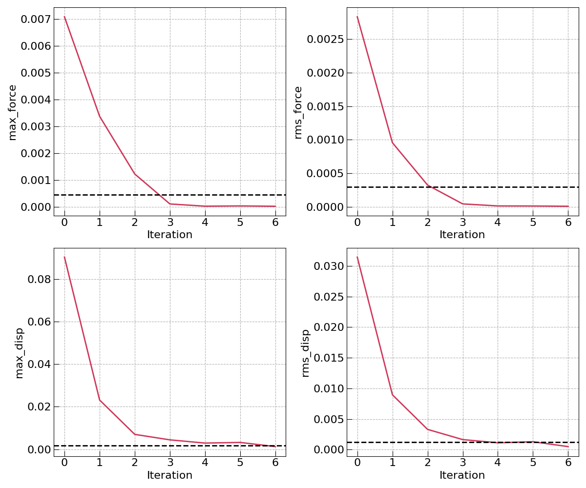
Inside the Optimization, Frequency, and ESP subdirectories, you
will find the Gaussian input and output files for the corresponding step. Inside the
Optimization subdirectory, you will also find a “convergence.png” figure that
shows the forces and displacement convergence during the course of the optimization.
The analysis subdirectory contains the results of the workflow in the form of a
esp.json file. You can read the content of the esp.json file using the
following commands:
1 2 3 4 5 6 | |
This will output the partial charges on the atoms of the molecule:
{
"1": ["O", -0.374646],
"2": ["O", -0.373831],
"3": ["C", 0.132166],
"4": ["C", 0.132716],
"5": ["C", 0.034284],
"6": ["C", 0.031733],
"7": ["H", 0.033853],
"8": ["H", 0.034024],
"9": ["H", 0.034218],
"10": ["H", 0.034388],
"11": ["H", 0.070724],
"12": ["H", 0.03474],
"13": ["H", 0.03438],
"14": ["H", 0.034621],
"15": ["H", 0.071656],
"16": ["H", 0.034974],
}